Regression

• Simple Linear Regression
• Best Fit Line
• Understanding Parameters \(b_0\) and \(b_1\)
• Common Error Variance
• Coefficient of Determination, \(r^2\)
• Pearson Correlation Coefficient, \(r\)

Simple Linear Regression

It is a statistical method to analyse the relationship between two continuous (quantitative) variables. One variable, denoted as x, is regarded as predictor, independent variable. Other variable denoted by y is known as response, dependent or target variable.

It is termed as simple because it involves only one predictor, in contrast with multiple linear regression which involves more than one predictor.

With machine learning aspect, we solve statistical relationship rather than deterministic relationship like relationship between celsius and fahrenheit, which is determined by equation F = (9/5)C + 32.

Statistical Relationship

Relationship between variables where the statistical uncertainty is present. For instance, relation between skin cancer mortality and state latitude. Below, we can see there is negative linear relationship between latitude and skin cancer mortality. Though its not a perfect linear relationship, it forms a trend.

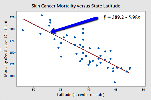
Figure 1: Skin Cancer Mortality vs Latitude

Similar statistical relationship can be found in following instances

• Height and weight.
• Driving Speed and gas mileage.

In the above figure, the linear line is the hypothesis.

Best Fit Line

In linear regression, we are solving for parameters with x and y, to find the relationship between them. Here, this relationship is translated into best fit line between the parameters, x and y. but how to find the best fit line?. Lets understand the plot between weight (y) and height (x).

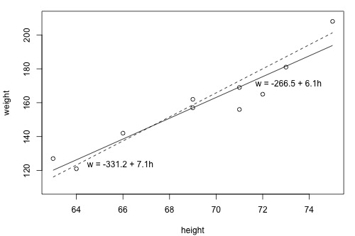
Figure 2: Approx. Best Fit Lines

$$ y^{`}_i = b_0 + b_1 x_i \\ \\ x_i - predictor\ value \\ y^{`}_i - predicted\ response \\ b_0,\ b_1 - parameters $$

In the above plot, we can see the multiple line equations with different set of parameters and each representing an approximate line of fit. Lets consider the line equation y = -266.5 + 6.1 x. For first sample, x=63, we find y` as 120.1, which is 6.9 less than ground truth value.

The difference between y and y` is referred as prediction error or residual error.

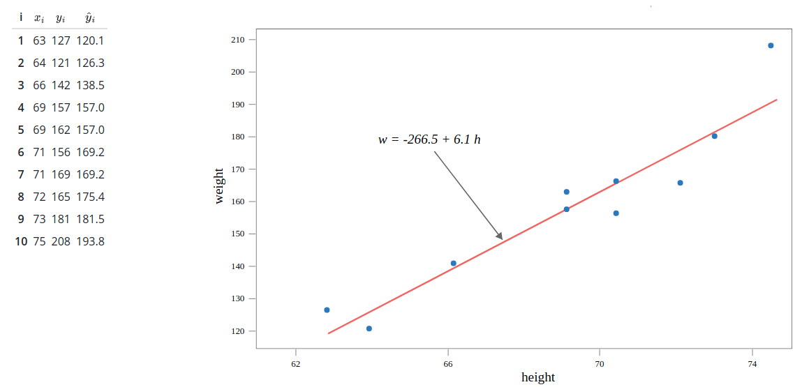
Figure 3: Best Line Fit

Prediction error depends on the data point, consider sample five, x = 69, whose weight (y) is not available. On substituting, x = 69, we find y`as 157 pounds, thus we get a prediction error of 162 - 157 = 5.

A line that fits the data “best” will be one for which the n prediction errors — one for each observed data point — are as small as possible in some overall sense. We can find the best fit line by using the least square criterion, which minimizes the sum of the squared prediction errors.

$$ Error\ = \ {\sum_{i=1}^n}\ (y_i\ -\ y_i^`)^2 $$

Why square the prediction error?

For each data point, we’ll have positive and negative prediction error. If we don’t square the prediction error, we’ll end up cancelling the positive and negative prediction error yielding zero as the net result.

Formulation of Best Fit Line

Lets check how the other line fits and its corresponding prediction error.

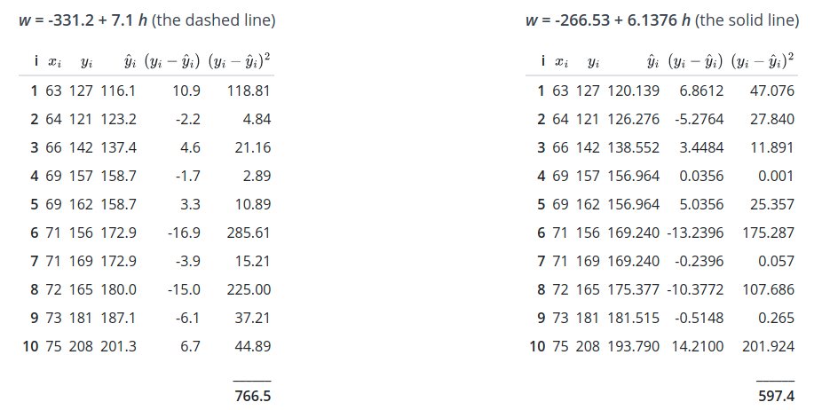
Figure 4: Error Difference Between Two Lines

For dashed line, we get a prediction error of 766.5, while for the solid line, we get a prediction error of 597.4. We can point out from the prediction error that the solid line has better summarization of data point with smaller prediction error overall. But does this solid line represent the best line? No. Because there are n lines passing through the data points.

To formulate the best parameters (intercept \(b_0\) and slope \(b_1\)) for the line equation, a formula is determined using methods of calculus. We minimize the equation for the sum of the squared prediction errors:

$$ Error\ =\ \sum_{i=1}^n\ (\ y_i\ -\ (b_0\ +\ b_1\ x_i ))^2 $$

(that is, take the derivative with respect to \(b_0\) and \(b_1\), set to 0, and solve for \(b_0\) and \(b_1\)) and get the “least squares estimates” for \(b_0\) and \(b_1\):

$$ For\ finding\ parameter\ b_0: \\ b_0\ =\ y^`\ -\ b_1\ x^` \\ \\ For\ finding\ parameter\ b_1: \\ b_1\ =\ {\sum_{i=1}^n\ (x_i\ -\ x^`)\ (y_i\ -\ y^`) \over \sum_{i=1}^n\ (x_i\ -\ x^`)^2} \\ \\ x^`\ refers\ to\ mean\ value\ of\ x's. \\ y^`\ refers\ to\ mean\ value\ of\ y's. $$

The formula for \(b_0\) and \(b_1\) is derived from least squares criterion. The resulting equation:

$$ y^`\ =\ b_0\ +\ b_1\ x_i $$

is referred as least square regression line, or simply the least squares line. It is also called as estimated regression equation.

What is \(b_0\) and \(b_1\)?

\(b_0\), when x = 0, then y becomes -267 pounds, which is incorrect. Here, x = 0 is outside the scope of the model because it is not meaningful to have 0 inch height. For other instances, \(b_0\) refers to predicted mean response at x=0, otherwise, \(b_0\) is not meaningful.

\(b_1\), it represents that for every unit (inch) increase in height, the weight increases by 6.1.

What \(b_0\) and \(b_1\) estimates?

Consider we have a population sample of High School GPA and College Entrance test score.

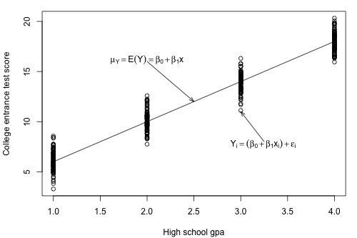
Figure 5: GPA vs Test Score

\(\mu_y\) is the estimate of population and the line is called as population regression line. From the above plot, we see that for each GPA score of 1, 2, 3, and 4, we see a corresponding set of test scores. We can also express the average college entrance test score for the \(i^{th}\) student, \(E(Yi)\ =\ β_0 +\ β_1\ x_i\). Of course, not every student’s college entrance test score will equal the average \(E(Yi)\). There will be some error. That is, any student’s response \(y_i\) will be the linear trend \(β_0\ +\ β_1\ x_i\) plus some error \(ϵ_i\). So, another way to write the simple linear regression model is \(y_i=E(Yi)+ϵ_i=β_0+β_1 x_i+ϵ_i\).

Practically it is impossible to get all the available data, thus we have to rely on taking the sub-population of the data and build a model on that sub-population. Let us take three random data point for each GPA score as mentioned in the plot below, thus resulting in a total of 12 data points.

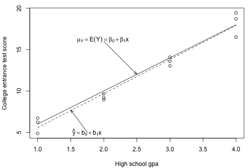
Figure 6: Plot sub-population

From above plot, the dashed line represents the sub-population regression line estimating the population regression line. Here, \(b_0\) and \(b_1\) represents the estimate of \(\beta_0\) and \(\beta_1\) from the population line. From sub-population line, we can draw some conclusions.

• For GPA score 1, the mean test score is 6. Few students did better to get a score of 9 and while few students got a score of 3. Instead of thinking of the error term \(\epsilon_i\), we can see majority of the errors are clustered near the mean of 0, with few as high as +3 and other as low as -3. If we could plot the curve, we can assume it should be normally distributed for each sub-population.
• We can look the spread of the error across each GPA, it will seem reasonable to assume that the variance of the error across each GPA is same.
• We can also conclude that the error for one student’s test score is independent of the error for another student’s test score.

We are now ready to summarize the four conditions that comprise “the simple linear regression model:”

• Linear Function: The mean of the response, \(E(Y_i)\), at each value of the predictor, \(x_i\), is a Linear function of the \(x_i\).
• Independent: The errors, \(ϵ_i\), are Independent.
• Normally Distributed: The errors, \(ϵ_i\), at each value of the predictor, \(x_i\), are Normally distributed.
• Equal variances (denoted \(σ^2\)): The errors, \(ϵ_i\), at each value of the predictor, \(x_i\), have Equal variances (denoted \(σ^2\)).

Common Error Variance

One of the conclusions made previously is that each sub-population have an equal variance denoted by \(\sigma^2\). It quantifies how much response \(y\) vary around the unknown mean population regression line \(\mu_Y\ =\ E(Y)\ =\ \beta_0\ +\ \beta_1\ x\).

Why \(\sigma^2\) is important? It helps in forecasting future response for unknown value of \(y\) using learnt \(\beta_0\) and \(\beta_1\).

Consider an experiment where we are measuring the temperature (Celsius) using two different brands of thermometer A and B. Below is the plot for converting these temperature from Celsius to Fahrenheit with estimated regression line for each brand.

For Brand A - Celsius vs Fahrenheit

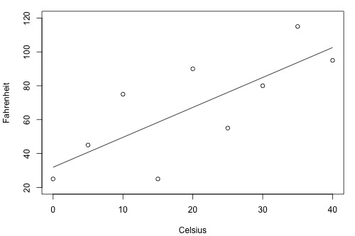
Figure 7: Brand A - Celsius vs Fahrenheit

For Brand B - Celsius vs Fahrenheit

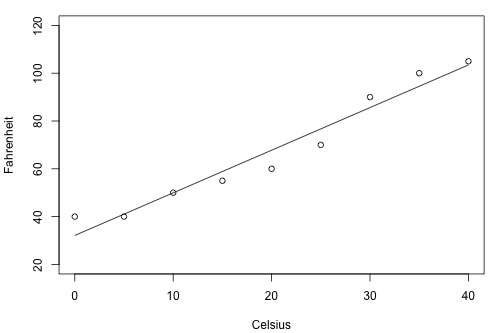
Figure 8: Brand B - Celsius vs Fahrenheit

Clearly from the above two plots, if we can make an estimation \(y^`\) based on brand B thermometer, then we’ll have less deviation from estimated regression line than compared to brand A thermometer. Therefore, brand B thermometer should yield more precise future predictions than the brand A thermometer.

To find how precise the future predictions are, we should know how much the response \((y)\) vary around the mean population regression line \(\mu_y\ =\ E(Y)\ =\ \beta_0\ +\ \beta_1\ x\). But we cannot estimate the value of \(\sigma^2\), which is population parameter, whose true value we’ll never know. The best is we can estimate it.

Let us understand, how variance is estimated from the below plot of IQ distribution. The population mean of the plot is at 100, how much does the IQ vary w.r.t to mean.

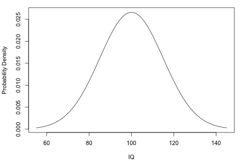
Figure 9: Distribution of IQ

Sample Variance

$$ s^2\ =\ {\sum_{i=1}^n\ (y_i\ -\ y^`)^2 \over n-1} $$

In numerator, we have summation of deviation of response \(y_i\) from \(y^`\) estimated mean in square units.

In denominator, we have n-1, not n since we are estimating \(y^`\), which reduces degree of freedom by one.

Mean Square Error

Let’s think about population variance \(\sigma^2\) in the simple linear regression setting. Previously, we have seen plot between GPA vs Entrance Test score. For each sub-population we have mean. Each sub-population mean can be estimated using regression equation \(y^`_i\ = b_0\ +\ b_1\ x_i\)

Mean Square Error

$$ MSE\ =\ {\sum_{i=1}^n\ (y_i\ -\ y^`_i)^2 \over n-2} $$

The mean square error estimates \(\sigma^2\), the common variance of the many sub-populations. Here, instead of n, we have n-2, because we are estimating two parameters \(b_0\) and \(b_1\), thus reducing the degree of freedom by two.

Coefficient Of Determination, \(r^2\)

Consider two different examples - each representing a relationship between x and y.

Weak relationship between x and y

Figure 10: Weak Relationship between x and y

In the above plot, there are two lines. One representing a horizontal line placed at the average response of \(\bar{y}\) and another line with shallow slope represents the estimated regression line \(\hat{y}\). Since slope is not steep, the change in predictor x doesn’t change much in response y. Even the data points are closer to regression line.

Some of the metrics to represent the relation between response and estimated response.

SSR - It refers to Sum of Square Regression. It quantifies how far the estimated regression line is w.r.t horizontal no relationship line, the sample mean or \(\bar{y}\).

SSE - It refers to Sum Of Square Errors. It quantifies how far the data points \(y_i\) vary from the estimated regression line \(\hat{y}\).

SSTO - It refers to Total Sum of Squares. It quantifies how far the data points \(y_i\) vary from their mean, \(\bar{y}\).

$$ SSR=\sum_{i=1}^{n}(\hat{y}_i -\bar{y})^2=119.1 \\ SSE=\sum_{i=1}^{n}(y_i-\hat{y}_i)^2=1708.5 \\ SSTO=\sum_{i=1}^{n}(y_i-\bar{y})^2=1827.6 $$

Note that SSTO = SSR + SSE. The sums of squares appear to tell the story pretty well. They tell us that most of the variation in the response y (SSTO = 1827.6) is just due to random variation (SSE = 1708.5), not due to the regression of y on x (SSR = 119.1). You might notice that SSR divided by SSTO is 119.1/1827.6 or 0.065.

Strong relationship between x and y

Figure 11: Fairly strong relationship between x and y

In the above plot, there is a fair amount relationship between x and y, with steeper slope of the regression line. It suggests that change (increase) in x leads to substantial change (decrease) in y. Here, we can see the data points touches the estimated regression line.

$$ SSR=\sum_{i=1}^{n}(\hat{y}_i-\bar{y})^2=6679.3 \\ SSE=\sum_{i=1}^{n}(y_i-\hat{y}_i)^2=1708.5 \\ SSTO=\sum_{i=1}^{n}(y_i-\bar{y})^2=8487.8 $$

Note The sums of squares for this data set tell a very different story, namely that most of the variation in the response y (SSTO = 8487.8) is due to the regression of y on x (SSR = 6679.3) not just due to random error (SSE = 1708.5). And, SSR divided by SSTO is 6679.3/8487.8 or 0.799.

Coefficient Of Determination or r-squared value

It is sum of square of regression divided by total sum of squares.

$$ r^2\ =\ {SSR\ \over SSTO}\ or\ 1\ -\ {SSE\ \over SSTO} $$

Characteristics of \(r^2\)

• \(r^2\) is always a number between 0 and 1.
• When \(r^2\ =\ 1\), all the data points fall perfectly on the estimated regression line. All predictor x accounts for variation in response y.
• When \(r^2\ =\ 0\), estimated regression line is horizontal. It means none of the predictor x accounts for variation in response in y.

In the above two examples, we had \(r^2\) value of 6.5% and 79.9%. We can interpret \(r^2\) as follows

”\(r^2\)×100 percent of the variation in y is reduced by taking into account predictor x”

”\(r^2\)×100 percent of the variation in y is ‘explained by’ the variation in predictor x.”

Note Here, x is associated with y, different from causation.

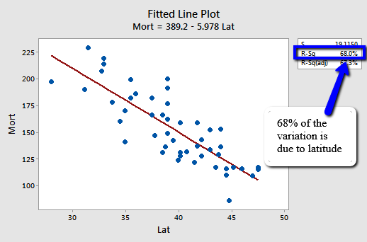
Figure 12: r-square value: Skin Cancer Mortality vs Latitude

We can say that 68% (shaded area above) of the variation in the skin cancer mortality rate is reduced by taking into account latitude. Or, we can say — with knowledge of what it really means — that 68% of the variation in skin cancer mortality is ‘due to’ or is ‘explained by’ latitude.

Pearson Correlation Coefficient \(r\)

It is directly related to coefficient of determination \(r^2\).

$$ r= \pm \sqrt{r^2} \\ where, \\ 0 \le\ r^2\ \le\ 1\ and\ -1 \le r^2 \le +1\\ $$

The sign of r depends on the sign of the estimated slope coefficient \(b_1\):

• If \(b_1\) is negative, then r takes a negative sign.
• If \(b_1\) is positive, then r takes a positive sign.

The slope of the estimated regression and the correlation coefficient has similar sign.

Correlation Coefficient, \(r\)

$$ r=\dfrac{\sum_{i=1}^{n}(x_i-\bar{x})(y_i-\bar{y})}{\sqrt{\sum_{i=1}^{n}(x_i-\bar{x})^2\sum_{i=1}^{n}(y_i-\bar{y})^2}} $$

• If the estimated slope \(b_1\) of the regression line is 0, then the correlation coefficient r must also be 0.

Interpreting \(r\) value

• If r = -1, then there is a perfect negative linear relationship between x and y.
• If r = 1, then there is a perfect positive linear relationship between x and y.
• If r = 0, then there is no linear relationship between x and y.

All other values of r tell us that the relationship between x and y is not perfect. The closer r is to 0, the weaker the linear relationship. The closer r is to -1, the stronger the negative linear relationship. And, the closer r is to 1, the stronger the positive linear relationship. As is true for the \(r^2\) value, what is deemed a large correlation coefficient r value depends greatly on the research area.

Reference

Penn State - Stat 501