Deploying a memory-intensive large deep model has a major downside if we’re planning to deploy these models in edge devices for real-time inference or systems with memory constraints. Edge devices have limited memory, computing resources, and power, which means a deep learning model must be optimized for this embedded deployment.

For instance, a simple network like AlexNet has a memory size of over 200 MB, while a network like VGG-16 has a memory size of over 500 MB. Networks of this size cannot fit on low-power micro-controllers and smaller FPGAs. To overcome such challenges, techniques like Quantization, Distillation is introduced.

In this blog post, we discuss Quantization and how it reduces the size of the model & the inference time with very small accuracy loss.

What is Quantization?

• It is a technique to perform computation on tensors and store the tensors in lower bit widths.
• Without quantization, the default datatype of the model parameter is float.
• Using quantization, we move the model parameters from float to an integer type.
• Changing parameter type from FP32 to INT8 reduces the memory by 4X.
• Quantized model executes some or all the operations in the tensor with integer values.

What Quantization does?

• It creates a compact size model
• It reduces the memory bandwidth required by 4X
• Hardware support for integer computation is 2x to 4x faster than FP32.
• Reduces the power consumed in transferring the data. Since energy consumption is dominated by memory access.
• Faster inference

Currently, Tensorflow and Pytorch natively support the quantization modules.

Two ways to use quantization

• Widely used approach, training on FP32 and convert it to INT8
• Running quantization aware training (available both in PyTorch and TensorFlow)

How quantization is done?

Conversion from float to int is the ultimate goal of quantization.

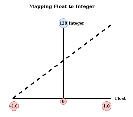
Figure 1: Float to Int

$$ x_{int} \ = \ {x_{float} \over x_{scale}} \ + \ x_{offset} $$

In a trained model, we’ll have parameters values in float between a range of floating-point numbers, and now we need to map these float numbers range to integer number range using the above mapping function.

Say the trained weights have a floating-point range in between -1.0 and +1.0. We create an integer range between 0 and 128. Now mark a point (-1.0, 0) and another point at (+1.0, 128), then draw a straight line connecting them. The inverse of the slope of the line is the scale, and the y value at the intersection of the line with x=0 is the offset, which is 64 (rounded from 63.5) in this example.

Dequantization is the reverse of quantization, multiply with scale and minus the offset to get back the floating-point number. We can see from the below sample, how during inference (eval), the model is quantized and dequantized.

Quantization - Pytorch Sample

        # Static Quantization also known as post-training quantization

        import torch

        # define a floating point model where some layers could be statically quantized
        class M(torch.nn.Module):
            def __init__(self):
                super(M, self).__init__()
                # QuantStub converts tensors from floating point to quantized
                self.quant = torch.quantization.QuantStub()
                self.conv = torch.nn.Conv2d(1, 1, 1)
                self.relu = torch.nn.ReLU()
                # DeQuantStub converts tensors from quantized to floating point
                self.dequant = torch.quantization.DeQuantStub()

            def forward(self, x):
                # manually specify where tensors will be converted from floating
                # point to quantized in the quantized model
                x = self.quant(x)
                x = self.conv(x)
                x = self.relu(x)
                # manually specify where tensors will be converted from quantized
                # to floating point in the quantized model
                x = self.dequant(x)
                return x

        # create a model instance
        model_fp32 = M()

        # model must be set to eval mode for static quantization logic to work
        model_fp32.eval()

        # attach a global qconfig, which contains information about what kind
        # of observers to attach. Use 'fbgemm' for server inference and
        # 'qnnpack' for mobile inference. Other quantization configurations such
        # as selecting symmetric or assymetric quantization and MinMax or L2Norm
        # calibration techniques can be specified here.
        model_fp32.qconfig = torch.quantization.get_default_qconfig('fbgemm')

        # Fuse the activations to preceding layers, where applicable.
        # This needs to be done manually depending on the model architecture.
        # Common fusions include `conv + relu` and `conv + batchnorm + relu`
        model_fp32_fused = torch.quantization.fuse_modules(model_fp32, [['conv', 'relu']])

        # Prepare the model for static quantization. This inserts observers in
        # the model that will observe activation tensors during calibration.
        model_fp32_prepared = torch.quantization.prepare(model_fp32_fused)

        # calibrate the prepared model to determine quantization parameters for activations
        # in a real world setting, the calibration would be done with a representative dataset
        input_fp32 = torch.randn(4, 1, 4, 4)
        model_fp32_prepared(input_fp32)

        # Convert the observed model to a quantized model. It does several things:
        # quantizes the weights, computes, and stores the scale and bias value to be
        # used with each activation tensor and replaces key operators with quantized
        # implementations.
        model_int8 = torch.quantization.convert(model_fp32_prepared)

        # run the model, relevant calculations will happen in int8
        res = model_int8(input_fp32)

Different Modes of Quantization

• Dynamic Quantization - Converting the weights to int8 happens in all quantization variants. But, converting the activations to int8 on the fly just before performing the computation is known as dynamic quantization.

The computations will thus be performed using efficient int8 matrix multiplication and convolution implementations, resulting in faster compute.

• Post-Training Static Quantization quantizes the weights and activations of the model. It fuses activations into preceding layers where possible. It requires calibration with a representative dataset to determine optimal quantization parameters for activations.

Post Training Quantization is typically used, when both the memory bandwidth and the compute savings are important. CNN network is a typical use case.

• Quantization-aware training(QAT) is the third method and the one that typically results in the highest accuracy of these three.

With QAT, all the weights and activations are fake quantized during both the forward and backward passes of the training. The float values are rounded to mimic the int8 values however all the computations are still done in floating-point numbers.

Thus, all the weight adjustments during training are made while “aware” of the fact that the model will ultimately be quantized; after quantizing, therefore, this method usually yields higher accuracy than the other two methods.

Performance Measure After Quantization

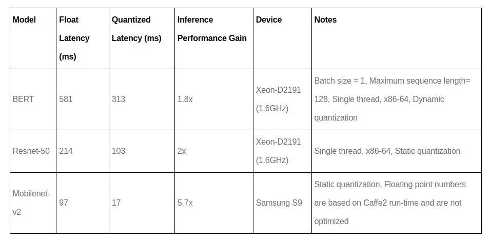
Figure 2: Performance After Quantization

We have just scratched the surface of quantization, it is a wide topic with variants of quantization. But we can get the idea that we can reduce our model inference time using quantization because the computation in type INT is faster than floating-point.

If you’ve liked this post, please don’t forget to subscribe to the newsletter.

Reference and more reading material

• Math behind Quantization
• Pytorch Quantization