ResNet

History

In 2010, Training a neural network was a computationally expensive task. But with the introduction of Deep Convolutional Network in AlexNet came techniques to reduce computation cost with efficient learning architectures.

In AlexNet, a set of concepts were utilized like Convolution Operation, Pooling, Non-Saturating Activation function, Local Response Normalization, and Dropout. The network implementation has five Conv layers and three fully connected layers, i.e., eight learning layers excluding the max-pooling and dropout layer.

With the current standing of neural networks in 2020, AlexNet sounds like a baby architecture but with parameters close to 65M neurons.

Anyway, when AlexNet was introduced, it managed to win all the major competition in the field of computer vision and reducing the test error rate by a great margin. Why Resnet then?

Challenges with Deep Networks

To build a deep neural network, we add more layers to the architecture, and its widely believed that by stacking more layers, the network learns better features for predictions.

So by adding more layers, we are learning better features, but during backpropagation, these learned parameters/gradients should pass through the same network and the gradients by the time it reaches the initial layers of the model becomes so small that it vanishes, causing Vanishing Gradient Problem.

Figure 1: Vanishing Gradient Problem

The next major issue with deep neural networks is the Degradation Problem. It means as the number of layers is increased, the training accuracy starts saturating and then degrading.

Consider a neural network with three layers (shallow network) with an 80% accuracy, and as mentioned earlier, that by stacking layers, the model learns better features.

We stack three more layers on this network, which only acts as identity mapping, i.e., f(x) = x, f is my identity function. Now, instead of retaining the same performance, the network starts degrading.

One way to look at this is that the network finds it difficult to map f(x)=x, and it would work better if f(x)=0, i.e., the shallow network.

In simple terms, the Degradation problem can be referred to as the inability to resolve the optimization for the deep network.

Resnet Breakthrough

In 2015, the Microsoft research team came up with the idea of Resnet. It found that splitting a deep network into three-layer chunks and passing the input into each chunk, straight through to the next chunk, along with the residual-output of the previous chunk, helped eliminate much of this Vanishing Gradient Problem and Degradation Problem.

No extra parameters or changes to the learning algorithm were needed. ResNets yielded lower training error (and test error) than their shallower counterparts simply by reintroducing outputs from shallower layers in the network to compensate for the vanishing data.

Note, ResNet is an ensemble of relatively shallow nets and does not resolve the vanishing gradient problem by preserving gradient flow throughout the entire depth of the network but rather, it avoids the problem simply by constructing ensembles of many short networks together.

On the ImageNet dataset, residual nets with a depth of up to 152 layers—8× deeper than VGG nets but still having lower complexity. An ensemble of these residual nets achieves a 3.57% error on the ImageNet test set. This result won 1st place on the ILSVRC 2015 classification task. We also present an analysis on CIFAR-10 with 100 and 1000 layers.

Resnet Block

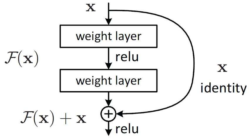
Figure 2: Resnet Block

How Resnet Functions works?

ResNet Block’s output is H(x) which is equal to F(x) + x. Assuming our objective function of Resnet Block is H(x). The author’s Hypothesize is that learning a function F(x) is simpler than H(x), and H(x) is a combination of input and output from a two-layered network. H(x) depends on F(x), which is the output of a two-layer network. F(x) is called Residual Mapping, and x is called Identity Mapping / Skip Connections.

The authors hypothesize that the residual mapping (i.e., F(x)) may be easier to optimize than H(x). To illustrate with a simple example, assume that the ideal H(x)=x. Then for a direct mapping, it is difficult to learn an identity mapping, as there is a stack of non-linear layers in between as follows.

x → weight1 → ReLU → weight2 → ReLU… → x

So, approximating the identity mapping with these weights and ReLUs in the middle would be difficult. Now, if we define the desired mapping H(x)=F(x)+x, then we just need to get F(x)=0 as follows.

x → weight1 → ReLU → weight2 → ReLU… → 0

Achieving the above is easy. Just set any weight to zero, and you will get a zero output. Add back x, and you get your desired mapping. Ultimately, we are trying to learn the parameters associated with F(x).

Backpropagation through Resnet

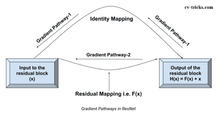
Figure 3: Backpropagation in ResNet

What happens during backpropagation

During backpropagation, the gradients can either flow through f(x) (residual mapping) or get directly to x (identity mapping).

If gradients pass through the residual mapping (gradient pathway 2), then it has to pass through the relu and conv layers. This Mapping can either make the value small or vanish the gradients.

Here, Identity Mapping comes into the picture, it directly moves the gradient to the initial layer skipping the residual mapping. Solving the Vanishing Gradient Problem.

Identity Mapping

Identity Mapping is also known as Skip Connections. It has been experimented widely by different elements like Dropout, Conv1x1 or multiplying with a constant factor, etc. Check out the identity mapping paper.

These experiments with various skip connections show varied results, i.e., find in the second image below.

The best result is obtained by plain mapping of x (identity shortcut) without any multiplicative manipulations like (scaling, gating, 1×1 convolutions, and dropout) on the shortcuts because such shortcuts can hamper information propagation and lead to optimization problems.

Note that the gating and 1×1 convolutional shortcuts introduce more parameters, and will have stronger representational abilities than identity shortcuts. The shortcut-only gating and 1×1 convolution cover the solution space of identity shortcuts (i.e., they can be optimized as identity shortcuts).

However, their training error is higher than that of identity shortcuts indicating that the degradation of this model is caused by optimization issues instead of representational abilities, which is why the degradation problem existed in the first place.

Experiments with Identity Mapping

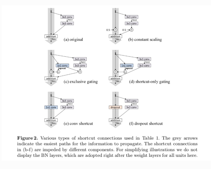
Figure 4: Identity Mapping

Results of Identity Mapping

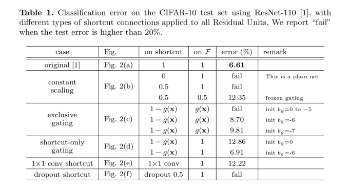
Figure 5: Result

Assumption about the Identity Mapping

No parameters are learned in identity mapping, i.e., when dimension matches between F(x) and x.

Since we are adding F(x) + x, the dimensions should match. If the dimensions don’t match, we can follow the below techniques to match the dimensions.

Either we can pad zeros to dimension to match F(x) with x or vice-versa.
We can use the conv1x1 layer, reduce or increase the dimensions. It introduces parameters and which in turn increases the time complexity.

In Conclusion

Resnet helps in building large neural networks by ensembling short resnet blocks.

Resnet solves Vanishing Gradient Problem by adding identity mapping.

Resnet solves the Degradation Problem by learning Residual Mapping F(x).

Resnet34 Implementation Using Pytorch

Loading Libraries

        import torch
        import torch.nn as nn
        import torch.nn.functional as F
        import torch.optim as optim
        from torchvision import transforms
        import torchvision
        import time

Creating DataLoaders and applying transforms on CIFAR10 Dataset

        transform = transforms.Compose([transforms.ToTensor(),
                            transforms.Normalize((0.5, 0.5, 0.5),(0.5, 0.5, 0.5))])
        trainset = torchvision.datasets.CIFAR10(root='/home/mayur/Desktop/Pytorch/data',
                            train=True,download=True, transform=transform)
        testset = torchvision.datasets.CIFAR10(root='/home/mayur/Desktop/Pytorch/data',
                            train=False, download=True, transform=transform)

        trainloader = torch.utils.data.DataLoader(trainset, batch_size=32,
                                                shuffle=True, num_workers=2)
        testloader = torch.utils.data.DataLoader(testset, batch_size=32,
                                                shuffle=False, num_workers=2)

Training on 2 Class of CIFAR10

        label_map = {0: 0, 2: 1}
        class_names = ['airplane', 'bird']
        cifar_2 = [(img, label_map[label1]) for img, label1 in trainset if label1 in [0,2]]
        cifar2_val = [(img, label_map[label]) for img, label in testset if label in [0, 2]]

        trainloader = torch.utils.data.DataLoader(cifar_2, batch_size=64,shuffle=True)
        testloader = torch.utils.data.DataLoader(cifar2_val, batch_size=64,shuffle=False)

        device = torch.device('cuda:0' if torch.cuda.is_available else 'cpu')
        """
        Files already downloaded and verified
        Files already downloaded and verified
        """

Train Function

        def train(model, optimizer, loss_fn, trainloader, testloader, n_epochs, device):
            for epoch in range(1, n_epochs+1):
                training_loss = 0.0
                valid_loss = 0.0
                
                model.train()
                for batch in trainloader:
                    img, label = batch
                    img = img.to(device)
                    label = label.to(device)
                    
                    output = model(img)
                    #print(output.shape)
                    optimizer.zero_grad()
                    loss = loss_fn(output, label)
                    loss.backward()
                    optimizer.step()
                    training_loss += loss.data.item()
                training_loss /= len(trainset)
                
                model.eval()
                num_correct = 0
                num_examples = 0
                for batch in testloader:
                    img, label = batch
                    img = img.to(device)
                    label = label.to(device)
                    
                    output = model(img)
                    loss = loss_fn(output, label)
                    valid_loss += loss.data.item()
                    correct = torch.eq(torch.max(F.softmax(output),dim=1)[1], label).view(-1)
                    num_correct += torch.sum(correct).item()
                    num_examples += correct.shape[0]
                    
                valid_loss/=len(testset)
                
                print(f'Epoch: {epoch}, Training Loss: {training_loss:.3f}, 
                Validation Loss: {valid_loss:.3f}, Accuracy: {num_correct/num_examples}')

Conv1x1

The purpose of using Conv1x1 is to make the dimension match between mapping function F(x) and x or h(x), as mentioned in the identity mapping paper. As mentioned in referenced links, Conv1x1 helps in decreasing or increasing the number of feature maps, i.e., it helps in dimension matching between resnet mapping and identity mapping.

1x1 is the kernel size of the convolutional operation. Conv1x1 is a projection shortcut, i.e., it comes into the picture when F(x) and x dimensions differ. Otherwise, Identity Mapping is done, without Conv1x1. Conv1x1 increases the time complexity because of the parameters to learn.

        def conv1x1(in_planes, out_planes, stride=1):
            return nn.Conv2d(in_planes, out_planes, kernel_size=1, stride=stride, bias=False)

Conv3x3 is a simple convolution operation on feature maps and inputs (x).

        def conv3x3(in_planes, out_planes, stride=1, padding=1):
            return nn.Conv2d(in_planes, out_planes, kernel_size=3, stride=stride, padding=padding)

Resnet Block

It contains 2 Conv with 1 Relu and 2 BatchNorm layers and downsamples layer. The network is simple to follow until it reaches to, downsample != None. Downsample is a sequential network with conv1x1 layer and batchNorm layer. (Think about Identity Mapping). The downsample layer is initialized when the feature map size is reduced to half (by stride=2), and it is compensated by increasing the number of filters by double.

Every time the number of filters increases from 64 to 128 then 128 to 256 and so on, the dimension changes throughout that combo of the block. When the number of filters is doubled, the downsample will make sure the identity x is also changed w.r.t to some filters to match the dimension.

Resnet Block

        class ResnetBlock(nn.Module):
            expansion = 1

            def __init__(self, inplanes, planes, stride=1, downsample=None, norm_layer=None):
                super().__init__()
                if norm_layer is None:
                    norm_layer = nn.BatchNorm2d
                self.conv1 = conv3x3(inplanes, planes, stride)
                self.bn1 = norm_layer(planes)
                self.relu = nn.ReLU(inplace=True)
                self.conv2 = conv3x3(planes, planes)
                self.bn2 = norm_layer(planes)
                self.downsample = downsample
                self.stride = stride

            def forward(self, x):
                identity = x

                out = self.conv1(x)
                out = self.bn1(out)
                out = self.relu(out)

                out = self.conv2(out)
                out = self.bn2(out)

                if self.downsample is not None:
                    identity = self.downsample(x)

                out += identity
                out = self.relu(out)

                return out

Explaining One Resnet Block

The below image is a sequential module with a resnet block. It is the second layer of the resnet network. In Layer 2, the resnet block, the input channel(feature map) is 64, and the output channel is 128.

Since the output channel is changed from 64 to 128, we need to change our identity mapping to meet the dimension of this output channel. After the residual mapping is done as mentioned in the paper, F(x), we bring in conv1x1 through the downsampling layer.

The downsample layer takes in input channel 64 but outputs channel 128 such that addition can take as mentioned above out+= Identity.

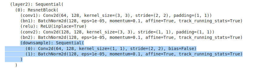
Figure 6: Downsample

ResNet34 Architecture

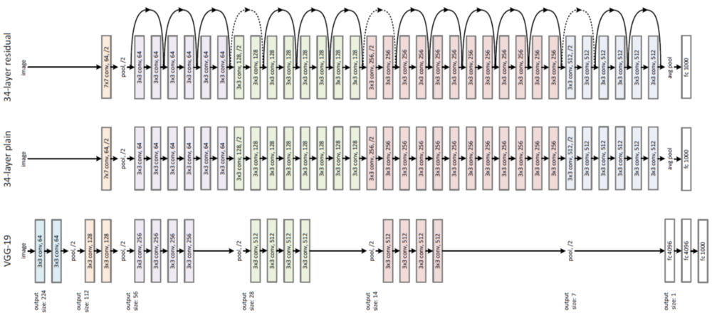
Figure 7: Resnet Architecture

Resnet Model Implementation

        class ResNet(nn.Module):

            def __init__(self, block, layers, num_classes=2,
                        norm_layer=None):
                super(ResNet, self).__init__()
                if norm_layer is None:
                    norm_layer = nn.BatchNorm2d
                self._norm_layer = norm_layer
                self.inplanes = 64
            
                self.conv1 = nn.Conv2d(3, self.inplanes, kernel_size=7, stride=2, padding=3, bias=False)
                self.bn1 = norm_layer(self.inplanes)
                self.relu = nn.ReLU(inplace=True)
                self.maxpool = nn.MaxPool2d(kernel_size=3, stride=2, padding=1)
                self.layer1 = self._make_layer(block, 64, layers[0])
                self.layer2 = self._make_layer(block, 128, layers[1], stride=2)
                self.layer3 = self._make_layer(block, 256, layers[2], stride=2)
                self.layer4 = self._make_layer(block, 512, layers[3], stride=2)
                self.avgpool = nn.AdaptiveAvgPool2d((1, 1))
                self.fc = nn.Linear(512 * block.expansion, num_classes)

                # Weight Initialization of layers like conv, batchnorm and bias.
                for m in self.modules():
                    if isinstance(m, nn.Conv2d):
                        nn.init.kaiming_normal_(m.weight, mode='fan_out', 
                                                nonlinearity='relu')
                    elif isinstance(m, (nn.BatchNorm2d, nn.GroupNorm)):
                        nn.init.constant_(m.weight, 1)
                        nn.init.constant_(m.bias, 0)

            def _make_layer(self, block, planes, blocks, stride=1):
                norm_layer = self._norm_layer
                downsample = None
                if stride != 1 or self.inplanes != planes * block.expansion:
                    downsample = nn.Sequential(conv1x1(self.inplanes, planes * block.expansion, stride), 
                                norm_layer(planes * block.expansion))

                layers = []
                layers.append(block(self.inplanes, planes, stride, downsample, norm_layer))
                self.inplanes = planes * block.expansion
                for _ in range(1, blocks):
                    layers.append(block(self.inplanes, planes, norm_layer=norm_layer))

                return nn.Sequential(*layers)

            def _forward_impl(self, x):
                # See note [TorchScript super()]
                x = self.conv1(x)
                x = self.bn1(x)
                x = self.relu(x)
                x = self.maxpool(x)

                x = self.layer1(x)
                x = self.layer2(x)
                x = self.layer3(x)
                x = self.layer4(x)

                x = self.avgpool(x)
                x = torch.flatten(x, 1)
                x = self.fc(x)

                return x

            def forward(self, x):
                return self._forward_impl(x)

Downsample with Conv1x1 for projection shortcut when the dimension is changed.

Resnet Layers

        model = ResNet(ResnetBlock, [3, 4, 6, 3])
        ### Start training

        start = time.time()
        net = model
        optimizer = optim.Adam(net.parameters(), lr=0.001)
        net.to(device)
        train(net, optimizer, torch.nn.CrossEntropyLoss(), trainloader, testloader, n_epochs=5, device=device)
        end = time.time()
        print(end-start)

Result

        /opt/anaconda3/lib/python3.7/site-packages/ipykernel_launcher.py:32: 
        UserWarning: Implicit dimension choice for softmax has been deprecated. 
        Change the call to include dim=X as an argument.


        Epoch: 1, Training Loss: 0.001, Validation Loss: 0.001, Accuracy: 0.8445
        Epoch: 2, Training Loss: 0.001, Validation Loss: 0.001, Accuracy: 0.838
        Epoch: 3, Training Loss: 0.001, Validation Loss: 0.001, Accuracy: 0.8605
        Epoch: 4, Training Loss: 0.001, Validation Loss: 0.001, Accuracy: 0.882
        Epoch: 5, Training Loss: 0.001, Validation Loss: 0.001, Accuracy: 0.899
        25.60597801208496

Total Parameters

        numel_list = [p.numel() for p in model.parameters()]
        sum(numel_list), numel_list

Details of AlexNet

AlexNet - 5 Conv, Pooling, 3 FC and Dropout.

Dropout - To reduce overfitting, the dropout drops neurons randomly in the layer.

The idea behind the dropout is similar to the model ensembles. Due to the dropout layer, different sets of neurons are switched off, with each representing a different architecture. And all these different architectures are trained in parallel with weight given to each subset and the summation of weights being one.

For n neurons attached to dropout, the number of subset architectures formed is 2^n. So it amounts to prediction, that being averaged over these ensembles of models. It provides a structured model regularization which helps in avoiding over-fitting.

Another view of dropout is that since the neurons are randomly chosen they tend to avoid developing co-adaptations among themselves, thereby enabling them to develop meaningful features, independent of others.

Relu - Non-saturating nonlinearity helps in reducing the time taken to train the model. It is better than Tanh and Sigmoid in terms of speed. The advantage of the ReLu over sigmoid is that it trains much faster than the latter because the derivative of the sigmoid becomes very small in the saturating region and therefore the updates to the weights almost vanish. This is called the vanishing gradient problem.

Convolution - It assumes the Stationarity of Statistics and the Locality of Pixel Dependencies.

Parameters - CNN has lesser parameters than FeedForward Neural Networks.

Local Response Normalization - This layer is used after relu because the relu gives out unbounded activation, and we normalize that. If we normalize around the local neighborhood of the excited neuron, it becomes even more sensitive as compared to its neighbors. LRN exhibits Lateral Inhibition.

In neurobiology, there is a concept called lateral inhibition. Lateral Inhibition refers to the capacity of an excited neuron to subdue its neighbors. We want a significant peak so that we have a form of local maxima. It tends to create a contrast in that area, hence increasing the sensory perception. Increasing sensory perception is a good thing since we want to have the same thing in our CNNs.

Pooling - It summarizes the output of a neighboring group of neurons in the same kernel map.

If you’ve liked this post, please don’t forget to subscribe to the newsletter.

References